Multitask Learning with Stochastic Interpolants

Hugo Negrel¹, Florentin Coeurdoux¹, Michael Albergo², Eric Vanden-Eijnden^{1, 3}

¹Capital Fund Management ²Society of Fellows, Harvard University ³Courant Institute of Mathematical Sciences, New York University, New York

Spotlight NeurIPS 2025

Paper arXiv Code

TL;DR This paper generalizes and extends the stochastic interpolant formalism to solve a very large variety of tasks with one single trained model. It provides zero-shot versatility; experimental validations include exact inpainting, editing, deblurring, constrained planning, as well as exact posterior sampling on high-dimensional datasets.

Abstract

We propose a framework for learning maps between probability distributions that broadly generalizes the time dynamics of flow and diffusion models.

To enable this, we generalize stochastic interpolants by replacing the scalar time variable with vectors, matrices, or linear operators, allowing us to bridge probability distributions across multiple dimensional spaces.

This approach enables the construction of versatile generative models capable of fulfilling multiple tasks without task-specific training. Our operator-based interpolants not only provide a unifying theoretical perspective for existing generative models but also extend their capabilities. Through numerical experiments, we demonstrate the zero-shot efficacy of our method on conditional generation and inpainting, fine-tuning and posterior sampling and multiscale modeling, suggesting its potential as a generic task-agnostic alternative to specialized models.

Key Contributions

Generalized stochastic interpolants: We replace the scalar time with linear operators to interpolate between distributions across dimensions. This points toward a more general paradigm of universal generative models that can be trained once and then applied to a variety of objectives.

Unified Generative framework: We provide a single formalism for multitask generation with flows and diffusions, without any sort of retraining.

zero-shot versatility: Perform conditional generation, inpainting, fine-tuning, and posterior sampling with one single model. You can impose hard constraints on the data generation, or make multiple generation in a row, one after another.

Universal generative models: Amortize training across tasks for scalable, task-agnostic generation. Inpainting and conditional generation can be performed during the same diffusion, saving time and computing resources.

Results

Inpainting

Consider images from high-dimensional image datasets CelebA and AFHQ-Cat. With multitask stochastic interpolants, pixel-wise inpainting becomes a trivial, one-shot task. Here, we consider block and random masking, probing two radically different inpainting situation.

Dataset: AFHQ-Cat

Original image

Block masking

Random masking

Dataset: CelebA

Original image

Block masking

Random masking

PSNR and SSIM metrics on CelebA and AFHQ-Cat datasets. A single generation was performed on each image. The best result of each category is highlighted in bold font.

Method	CelebA				AFHQ-Cat
	Random		Block		Random		Block
	PSNR	SSIM	PSNR	SSIM	PSNR	SSIM	PSNR	SSIM
Degraded	11.82	0.197	22.12	0.742	13.35	0.234	21.50	0.744
pokle2024trainingfree	28.36	0.865	28.84	0.914	28.84	0.838	23.88	0.874
hamu2024dflow	33.07	0.938	29.70	0.893	31.37	0.888	26.69	0.833
zhang2024flow	32.33	0.945	29.40	0.858	31.76	0.909	25.85	0.822
martin2024pnp	33.54	0.953	30.59	0.943	32.98	0.930	26.87	0.904
Ours	33.76	0.967	29.98	0.938	33.11	0.945	26.96	0.914

Of all the inpainting benchmarks, multitask stochastic interpolants perform best while offering great flexibility, both on PSNR and SSIM metrics. The very same model is employed for both block and random inpainting.

The eyes and mouth are masked then generated in turn. Multiple generations are performed in a row on the same image. The final result does not deviate significantly from the original image, see below.

Original image

Masked eyes

Generated eyes

Generated eyes + Masked mouth

Generated eyes + Generated mouth

Original image

Masked eyes

Generated eyes

Generated eyes + Masked mouth

Generated eyes + Generated mouth

Generation flow

Constrained planning

This problem takes root in Reinforcement Learning (RL). Take a maze and two end points. The task is to find the shortest path joining them while abiding by the contraints imposed in the environment. With stochastic interpolants, to generate a path, you simply fix the first and last point, and eventually let diffuse all other intermediates points.

The constraints do not necessarily have to apply only on the end points, you can also impose hard constraints on the pathway, assuming it remains feasible. A small white dot represents the constraints applied on the path, forcing it to take a detour. The path length adapts accordingly.

Shortest path, no constraint except end-points.

Path under a constraint at mid-length, here on the bottom-right corner.

Posterior sampling

With the very same model, you can perform exact posterior sampling. Take the $\varphi^4$ model. Consider the system with energy $E$ under a null magnetic field and assume a field configuration can be sampled with coefficients $\alpha$ and $\beta$. It yields the prior distribution. Now, consider the same system under a magnetic field $h$, its energy becomes $E_r=E + (h, \varphi)$. By simply shifting the field configuration during generation process: $\varphi_r=\varphi + \frac{\alpha^2}{\beta} h$, you can sample from the posterior without retraining or any kind of approximation. The training data was generated with Hamiltonian MCMC. The figure below shows that stochastic interpolants generate data that reproduce the magnetisation statistic $M(\varphi) = \frac1N \sum\limits_{a} \varphi(a)$ for $h = 0$ and $h \ne 0$ with a single model.

Model: $\varphi^4$

A major limitation of HMC methods in very high dimension is the low acceptation rate of sampling a new configuration after reaching the stationary distribution. Consequently, generating a whole dataset of $\varphi^4$ configuration is therefore time-consuming. With our method, sampling a configuration close to an other is trivial, you can just mask out a subset of spins, and generate them again immediately, as illustrated below!

Block masking

Theoretical Framework

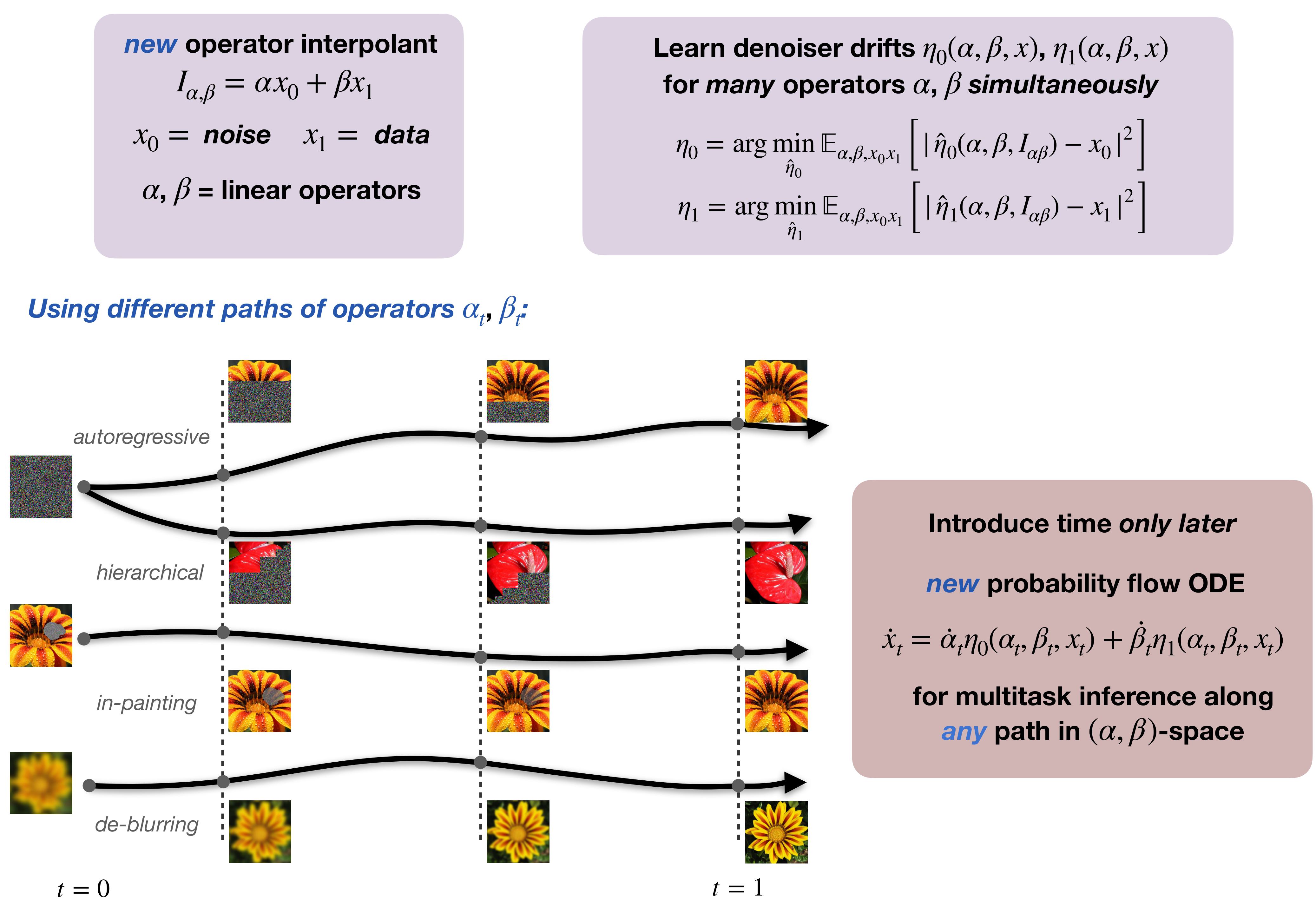
New operator interpolant
$$ \begin{align*} I_{\alpha,\beta}(x_0, x_1) = \alpha x_0 + \beta x_1, \end{align*} $$ where $x_0 \sim$ noise, $x_1\sim$ data distribution and $\alpha,\beta$ are linear operator.

Associated with this interpolant we introduce:

Denoiser drifts:
$$ \begin{align*} \eta_0(\alpha,\beta,x) = \mathop{\mathrm{arg min}}\limits_{\hat \eta_0} \mathbb{E}_{x_0,x_1,\alpha,\beta}\big[|\hat \eta_0(\alpha,\beta,I_{\alpha,\beta})- x_0|^2\big], \\ \eta_1(\alpha,\beta,x) = \mathop{\mathrm{arg min}}\limits_{\hat \eta_1} \mathbb{E}_{x_0,x_1,\alpha,\beta}\big[|\hat \eta_1(\alpha,\beta,I_{\alpha,\beta})- x_1|^2] \end{align*} $$

These drifts can be used to perform inference along any path in $(\alpha,\beta)$-space using:

Probability flow ODE
$$ \begin{align*} \dot x_t = \dot \alpha_t \eta_0(\alpha_t,\beta_t,x_t) + \dot \beta_t \eta_1(\alpha_t,\beta_t,x_t), \qquad x_0 \overset{d}{=} I_{\alpha_0,\beta_0} \end{align*} $$ SDE
$$ \begin{align*} dx_t = (\dot \alpha_t -\sigma_t^{2} \alpha_t^{-1})\eta_0(\alpha_t,\beta_t,x_t) dt + \dot \beta_t \eta_1(\alpha_t,\beta_t,x_t) dt + \sqrt{2} \sigma_t dW_t, \qquad x_0 \overset{d}{=} I_{\alpha_0,\beta_0}\end{align*} $$

In terms of sampling, solving the SDE or ODE is strictly equivalent, that is, $Law(x_t)^{SDE} = Law(x_t)^{ODE}$. The only difference lies in the numerical method employed; an Euler or an Euler-Maruyama scheme respectively.

The heart of the message is that a single trained model can perform multiple tasks of very different natures, which are uniquely specified by the $(\alpha_t, \beta_t)_{t \in [0, 1]}$-path.

BibTeX

@article{negrel2025multitasklearningstochasticinterpolants,
        author    = {Negrel, Hugo and Coeurdoux, Florentin and Albergo, Michael and Vanden-Eijnden, Eric},
        title     = {Multitask Learning with Stochastic Interpolants},
        journal   = {NeurIPS2025},
        year      = {2025},
        url       = {https://arxiv.org/abs/2508.04605}
                }